Fold hinges-faults intersections analysis is suitable for regions characterised by a lack of outcrops and weak seismic activity. It provides data on fault kinematics and stress fields based on the 3D seismic interpretation without additional information from wells. The results are used for tectonic history, fracture modelling, fault seal behaviour and fault reactivation potential.
The analysis has been tested on three study areas with different tectonic stress regimes. At first on the Archinsk oilfield in the West Siberian Basin (Moskalenko et al., 2020; Moskalenko and Khudoley, 2020), then on the Kuyumba oilfield in the Siberian Craton (Moskalenko et al., 2017; Moskalenko, 2017), and later on the Novoport oilfield in the Yamal Peninsula.
I thank professor Andrey Khudoley (St Petersburg University) for working together on the fold hinges-faults intersections analysis and for discussing its fundamental principles. I am very grateful to have worked under his supervision.
Please refer to the following publication for more details:
Moskalenko A., Khudoley A., and Cardozo N., 2020. Fault kinematics and paleostress analysis using seismic data: A case study from the Archinsk field, West Siberian Basin, Russia // Journal of Structural Geology 141, 104194
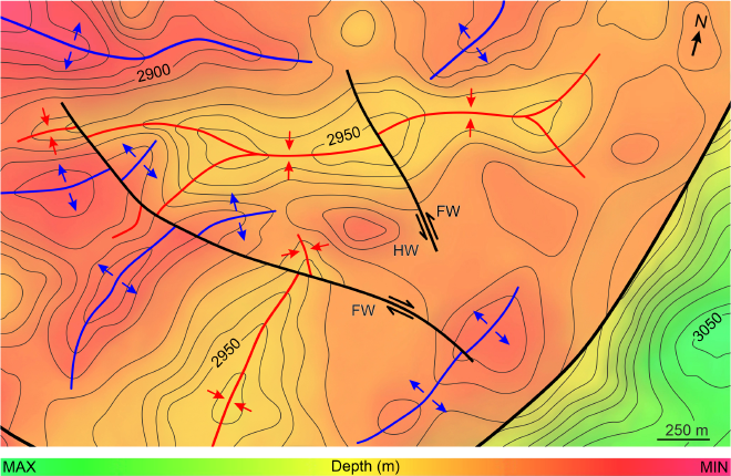
To perform the analysis, depth-converted 3D seismic reflection data are required, that should include at least two seismic horizons and several fault surfaces that post-date the folds. A good example of the fold-fault relationships is shown in Fig. 1, where two NW-trending strike-slip faults with right-lateral and left-lateral slip components offset anticlinal and synclinal structures on the surface of seismic horizon.
Figure 1. Structure map of portion of seismic horizon with contour interval = 10 m. The map shows that the faults post-date the folds. FW footwall, HW – hanging wall, blue and red lines are the fold hinges of anticlines and synclines, respectively.#
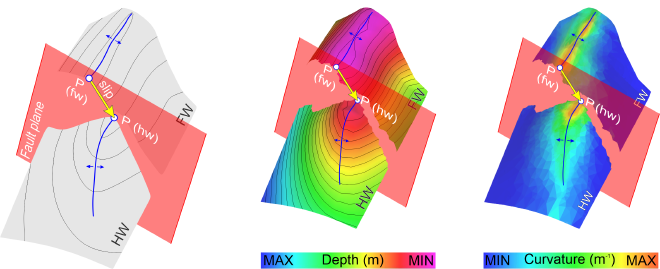
Fold hinges-faults intersections analysis is based on the study of the interpreted seismic horizons structure maps Fig. 2. Firstly, the hinge line of a fold structure, such as an anticline or syncline (Lisle and Toimil, 2007) is identified on the seismic horizon. This fold hinge is offset by a fault and its intersections on both the footwall and hanging wall mark the piercing points, used to calculate the trend, plunge, rake and displacement of the fault slip vector following Allmendinger et al. (2012). Finally, the strike, dip and sense of slip of the fault plane containing the slip vector are calculated. Analysis of the structure maps’ geometry identifies the fold hinges. The curvature analysis (Pollard and Fletcher, 2005) is used to identify them, whether the maximum and minimum curvature values on the seismic horizons correspond to the fold hinges of anticlines and synclines, respectively. The higher are the values of the principal curvature, the more reliable and precise is selection of the piercing points.
Figure 2. Structure map analysis and interpretation of the slip vector on the fault plane. The fold hinge (blue line) defines piercing points (P) on the footwall (fw) and hanging wall (hw) sides of the fault. These intersections define the fault slip vector (yellow arrow). From left to right they are: synthetic model; analysis of the surface geometry; and curvature analysis of the surface.#
The determination of anticlinal and synclinal fold hinges on seismic horizons might not be accurate, even though both the structure map geometry and curvature analyses are used. Moreover, the fold hinges-faults intersections indicate the total displacements that may correspond to one or more stress regimes. Hence, data quality control is important for preparing the final dataset of the fault planes and slip vectors. The quality control consists of two requirements. The first is that the slip vector orientation and the magnitude should vary gradually along the same fault surface on each seismic horizon. The fault-slip dataset does not contain measurement points where there are drastic changes of the slip vector (e.g. from left-to right-lateral slip) on the same fault surface. The second is that the fault kinematics has to be uniform for the same fault segment on the different seismic horizons. After quality control, a heterogeneous fault-slip data are used for the paleostress analysis based on slip inversion methods (e.g. Gushchenko, 1979; Angelier, 1994; Nemcok and Lisle, 1995; Yamaji, 2000; Delvaux and Sperner, 2003; Thakur et al., 2020).
Fault kinematics are presented by orientation of faults (strike, dip direction and dip) and slip vectors (trend, plunge and rake), fault displacements (total, heave and throw) and sense of slip (normal faulting with left-lateral slip displacement, strike-slip fault, etc). Basically, a heterogeneous fault-slip dataset is based on a hundred or more displaced fold structures.
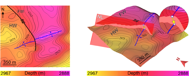
An anticline is identified on the seismic horizon as an example Fig. 3. Coordinates of the piercing points allow to calculate the slip vector orientation and displacement. In the example case, the fault orientation is 168°/85° (righthand-rule format). The slip vector orientation is (trend and plunge) 171°/39°, and the fault displacement is 37 m. The fault heave and throw are 29 m and 24 m, respectively. Thus, this locality is characterized by SSE-trending oblique-slip faults with left-lateral slip component and rake 39°S.
Figure 3. Fold hinge-fault intersection analysis of an anticline structure on the seismic horizon. Structure map with contour interval = 5 m. Oblique view of 3D model with vertical exaggeration = 3. The intersection of the fault surface and fold hinge (blue line) define the fault slip vector (yellow arrow). FW – footwall, HW – hanging wall.#
Fault displacement data distribution allows analysing changes in total displacement with depth. As an example, the Archinsk oilfield fault displacement vectors have estimated magnitude of 10–400 m that decreases from the deepest seismic horizon to the shallowest.
The rake of the fault slip vectors is used to separate the dip-slip and strike-slip faulting. Fault kinematics are similar in seismic horizons at 2.9 km, 2.8 km and 2.7 km, but they are different in seismic horizon at a depth of 3.1 km. Therefore, two fault populations can be defined: normal faulting and strike-slip faulting. The measurements of second fault population in all seismic horizons is characterised by strike-slip faulting:
In the chart above:
N – normal faulting
NL – normal faulting with left-lateral slip displacement
NR – normal faulting with right-lateral slip displacement
The direction of the maximum (σ1) and minimum (σ3) principal stresses, as well as, the shape of the stress ellipsoid (Φ) for each stress regime constitute the stress field data. Stress data obtained by full-bore formation microimager analysis (FMI by Shlumberger) is consistent with present-day stress regimes brought by fold hinges-faults intersections analysis.
For example, the following are the results of the paleostress analysis for the Archinsk field located in the SE part of the West Siberian Basin, close to the Central Asian Orogenic Belt.
The multiple inverse method was applied to all the 126 fault-slip vectors from all seismic horizons. Two stress regimes were identified by 89 fault-slip vectors based on the analysis of the minimal values of angular misfit for each stress ratio Φ. These fault-slip vectors correspond to either one of these stress regimes, but the slip vectors show different angular misfits. 37 fault-slip vectors or 29.4% of the fault-slip dataset do not fall in either of these stress regimes. The first stress regime corresponds to normal faulting and is represented by 48 fault-slip vectors. The second stress regime corresponds to strike-slip faulting and is represented by 65 fault-slip vectors.
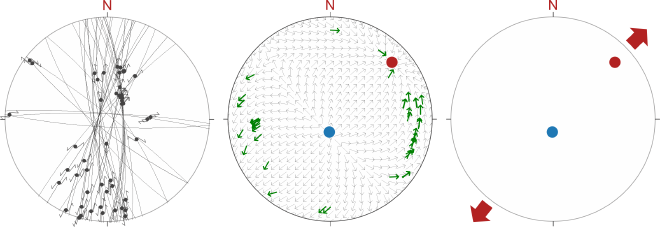
The “normal faulting” stress regime Fig. 4 corresponds to an extensional regime with a almost vertical σ1, a sub-horizontal NE-trending σ3, and Φ = 0.5. Slip vectors with angular misfits <30° are mostly identified on the deepest seismic horizon (33 out of 48 measurements).
Figure 4. The “normal faulting” stress regime. The results are shown on equal-angle lower-hemisphere projections. From left to right they are: homogeneous fault-slip data; tangent lineation diagrams showing the theoretical slip directions (grey arrows) and the movement of the hanging wall blocks (green arrows); and principal stresses orientations. Blue circle and arrows – σ1, red circle and arrows – σ3#
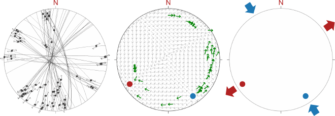
The “strike-slip faulting” regime Fig. 5 is characterized by sub-horizontal σ1 and σ3 with SE and SW- trend, respectively, and Φ = 0.3. The lowest values of angular misfit are mostly on shallowest seismic horizons (40 out of 65 measurements).
Figure 5. The “strike-slip faulting” stress regime. The results are shown on equal-angle lower-hemisphere projections. From left to right they are: homogeneous fault-slip data; tangent lineation diagrams showing the theoretical slip directions (grey arrows) and the movement of the hanging wall blocks (green arrows); and principal stresses orientations. Blue circle and arrows – σ1, red circle and arrows – σ3#
In the study area, the NW rift system suggests an approximately NE-SW orientation of σ3. Fault slip vectors and paleostress analysis for the deepest seismic horizon, corresponding to the surface of the basement, show an extensional regime with Φ = 0.5 and a NE-trending σ3. This supports the validity of analysis and implies that within the study area the Late Triassic-Early Jurassic stress field was inherited from earlier stages of the Triassic West Siberian rift system. The World Stress Map (Heidbach et al., 2018) does not display any data on the present-day stress for the study area and the wide region around. However, drilling-induced fractures in the Archinsk field indicate a NW-trending σ1 based on full-bore formation microimager analyses. The predominance of W-WNW-dipping sinistral strike-slip faults and SSW-SW-dipping dextral strike-slip faults on shallowest seismic horizons supports the NW-trending σ3 as well. The paleostress analysis in these horizons show strike-slip faulting, NW-trending σ1 and NE-trending σ3, and a transpressional tectonic regime with Φ = 0.3. The most likely interpretation for this similarity is that strike-slip faulting and the related state of stress shallowest seismic horizons reflect present-day stresses. Moreover, the estimated NW-trending σ1 from the fault slip inversion is related to the Cenozoic India-Eurasia collision and is consistent with the NNW direction of horizontal displacement GPS vectors in the West Altai from 2000 to 2012, with a rate of 1.2 mm/year (Timofeev et al., 2019). The present-day strike-slip tectonic setting is also recognized in the northern part of the West Siberian Basin (Sim and Bryantseva, 2007; Gogonenkov and Timurziev, 2012).
The fault seal behaviour is in controlling hydrocarbon accumulations. In this study, it is based on the dilation tendency analysis (Ferrill et al., 2019). Dilation tendency ranges between 0 and 1, where the higher value corresponds to likelihood of fault dilatation, which is controlled by the resolved normal stress acting on the surface of interest (σn). Dilation tendency (Td) was defined by Ferrill et al. (1999) as follows:
Consequently, the detailed kinematic evolution of fault systems and stress fields by the fold hinges-faults intersections analysis allows to determine different deformation styles that occur along the same faults, significantly affecting each fault’s ability to act as a conduit or barrier. As an example, the dilation tendency analysis at the normal and strike-slip faulting stress regimes in the Archinsk oilfield is presented.
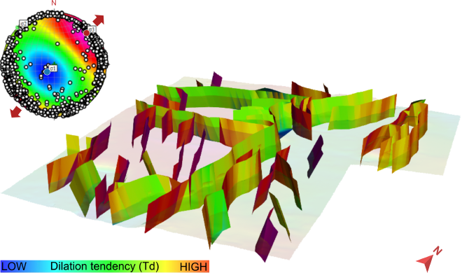
The Late Triassic-Early Jurassic extensional regime with a NE-trending σ3 is not characterised by faults as a barrier, as Td has mainly medium values Fig. 6.
Figure 6. Three-dimensional dilation tendency model of Archinsk fault system at the “normal faulting” stress regime with no vertical exaggeration. The poles to planes of faults are shown on equal-angle lower-hemisphere projection coloured according to dilation tendency as defined in the text. The deepest seismic horizon is presented.#
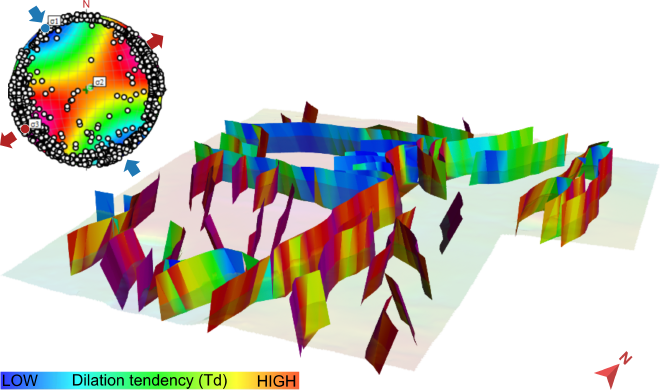
However, from the Eocene the tectonic stress regime changes to a transpressional regime with NW-trending σ1 and NE-trending σ3, where Fig. 7 E-trending oblique normal faults are barriers (Td is low) and NE-to N-trending sinistral strike-slip faults are conduits (Td is high).
Figure 7. Three-dimensional dilation tendency model of Archinsk fault system at the “strike-slip faulting” stress regime with no vertical exaggeration. The poles to planes of faults are shown on equal-angle lower-hemisphere projection coloured according to dilation tendency as defined in the text. The deepest seismic horizon is presented.#
Fault reactivation and hydrocarbon leakage could be caused by resolved shear stress (τ) to normal stress (σn) acting on fault surfaces. Slip tendency ranges between 0 and 1, where the higher value corresponds to likelihood of fault slip. Slip tendency (Ts), was defined by Morris et al. (1996) as follows:
$$
Ts = (\tau / \sigma_n)
$$
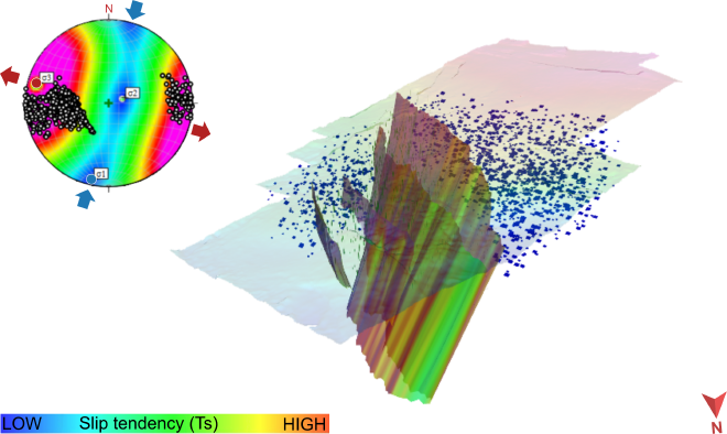
The application of the fold hinges-faults intersections analysis made it possible to determine the present-day stress field on the Novoport oilfield without additional expensive drilling. Furthermore, based on the slip tendency, analysis has allowed to find out the fault orientations that are nearly optimally oriented for a frictional slip in the present-day stress field Fig. 8. These results are useful for estimating the fault slippage and hydrocarbon leakage along sections of previously sealing reservoir-bounding faults.
Figure 8. Three-dimensional model of Novoport fault system with fault surfaces coloured according to slip tendency with vertical exaggeration = 2. The poles to planes of faults are shown on equal-angle lower-hemisphere projection coloured according to slip tendency as defined in the text. The shallowest seismic horizon and discrete fracture network are presented.#
Future work involves fracture modelling of the reservoirs based on the results of fold hinges-faults intersections analysis using 3D seismic reflection data.